








QIAGEN CLC Genomics Workbench provides tools and workflows for a broad range of bioinformatics applications, including microbiome analysis, isolate characterization through SNP and K-mer trees using NGS data, and antimicrobial resistance characterization. CLC Genomics Workbench is widely used for analyses of bacterial, viral and eukaryotic (fungal) genomes and metagenomes.
We’ll cover these topics in the training:
I. Overview of different tools within MGM application and research areas supported
II. Focused review of isolate typing and characterization
a. Importing data
b. Utilization of metadata
c. Downloading and managing references
i. Database of Isolates/ Resistances/ MLST
d. Walk through of Type a Known Species workflow
i. Review details for each Isolate
e. Creating SNP profiles to specific reference
f. Generate a SNP tree for isolate comparison
g. Export tabular and high-quality graphical outputs in wide range of file formats
Are you struggling to find a bioinformatics analysis tool that meets your specific research needs? One that is easy-to-use, yet powerful, scalable and flexible? We are excited to announce the launch of QIAGEN CLC Genomics 21.0, packed with new features to help you take your data analysis to the next level. QIAGEN CLC Genomics has solutions for all your sequencing, NGS and 'omics data analysis needs. Get the features that meet your research goals with our new licensing models developed for this v21 release. Our favorite new features and functions now available in v21 include:
Illumina BaseSpace integration Data stored in Illumina BaseSpace can now be seamlessly imported into the Workbench. To get started, just install the Cloud Plugin. Illumina BaseSpace will then be available to select as an import location.

Sanger workflows Draw end-to-end workflows for the analysis of Sanger reads, starting with on-the-fly import of trace files. If you run the trimming and assembly of forward-reverse Sanger reads in batch mode, the outputs will be named after the batch unit – or you can use advanced custom output naming patterns in workflows to include even more information in the file names. Extract consensus sequences and create alignments within the same workflow. You can now also visualize Sanger assemblies in the wrapped view.

New in the v21 release, QIAGEN CLC Genomics now has three key offerings, with packages ranging from basic (QIAGEN CLC Main Workbench), advanced (QIAGEN CLC Genomics Workbench) and premium (QIAGEN CLC Genomics Workbench Premium), to meet your specific sequence and ‘omics data analysis needs.
QIAGEN CLC Main Workbench: For basic sequencing analysis
QIAGEN CLC Genomics Workbench: For advanced sequencing analysis
Includes all the features of the QIAGEN CLC Main Workbench, plus:
QIAGEN CLC Genomics Workbench Premium: Our full-featured solution
Includes all the features of the QIAGEN CLC Genomics Workbench, plus:
QIAGEN CLC Genomics Server: All CLC functionality is also available as enterprise software, which operates on any hardware server. The Genomics Analysis Portal allows sample- and workflow centric views of analyses run on the server.
QIAGEN CLC Genomics Cloud Engine: Run CLC workflows in the cloud on data stored in your BaseSpace or AWS S3 account. Launch workflows from the CLC Genomics Workbench or Server in the cloud using the Cloud Plugin.
Learn more about the applications supported by our portfolio of QIAGEN CLC Genomics solutions, and request a consultation with one of our experts to help you find the right QIAGEN CLC toolset for your research goals.
This blog tutorial highlights several recent improvements in the latest update to QIAGEN CLC Microbial Genomics Module 20.1. The update includes improved usability in the Download Microbial Reference Database tool and improved support for long reads in Taxonomic Profiling. Some of the improvements include:
With the 20.1 update, it is now easy to customize the Microbial Reference Database to fit your needs. Here we demonstrate two use cases:
The updated downloader makes it simple to visualize phylogenetic relationships. To create a dendrogram of the four coronavirus genera, we first create a microbial database containing only coronavirus:
Approximately 200 references remained and were downloaded with a minimum contig length of 1000. The five samples with an unknown genus were included in the downloaded database.
The phylogenies of the downloaded database of assemblies can be easily visualized using Create K-mer Tree. In Create K-mer Tree, select the downloaded database of coronavirus genomes. The dendrogram shown was created with default settings, except "Only index k-mers with prefix" was left blank due to the short length of coronavirus genomes.
Figure 1 shows a circular dendrogram with added genus metadata. For ease of viewing, 50% of both the alphacoronavirus and betacoronavirus genomes have been excluded from the tree.
In the tree, the five references without a genus are selected and their branches are shown in dark blue. From the tree, we can see that three of these references cluster with the betacoronavirus, one clusters with the alphacoronavirus and one clusters between alphacoronavirus and gammacoronavirus.
This highlights a quick and easy way to download a database of viral genomes, and how to use the database to create a phylogeny. The phylogeny can then be used to resolve samples of unknown genus.

Create K-mer tree also works with reads. In the next section, we demonstrate how to create a taxonomic profile with metagenome samples.
With the recent updates to the Download Microbial Reference Database and Taxonomic Profiling functions in QIAGEN CLC Microbial Genomics Module, it is now fast and easy to detect coronavirus presence in metagenome samples containing only a few virus reads. Taxonomic profiling now also supports long reads such as those generated by Oxford Nanopore and PacBio sequencing technologies.
For the first time setup, we create a viral database:
All complete virus genomes to date, approximately 18,500, remained and were downloaded with a minimum contig length of 1000.
The downloaded database was used to create a taxonomic profiling index using default settings.
The analysis can be carried out in a simple workflow using the curated Microbial Reference Database and human genome to create a Taxonomic Profiling index for host genome filtering (Figure 2).

Results are presented from 3 different studies with low fraction of viral reads (Table 1).
Abundance virus values have been aggregated to species level and table filtered to abundance >10. The % viral reads is the percentage of reads in the sample matching the virus database.
| Sample | % viral reads | Species | Taxonomy | Abundance |
|
SRR10948550 |
1.0556 |
Severe acute respiratory syndrome-related coronavirus | Orthornavirae; Pisuviricota; Pisoniviricetes; Nidovirales; Coronaviridae; Betacoronavirus; Severe acute respiratory syndrome-related coronavirus | 985 |
| Ambystoma tigrinum virus | Bamfordvirae; Nucleocytoviricota; Megaviricetes; Pimascovirales; Iridoviridae; Ranavirus; Ambystoma tigrinum virus | 39 | ||
| Common midwife toad virus | Bamfordvirae; Nucleocytoviricota; Megaviricetes; Pimascovirales; Iridoviridae; Ranavirus; Common midwife toad virus | 26 | ||
|
SRR11092061 |
0.0045 |
Severe acute respiratory syndrome-related coronavirus | Orthornavirae; Pisuviricota; Pisoniviricetes; Nidovirales; Coronaviridae; Betacoronavirus; Severe acute respiratory syndrome-related coronavirus | 1304 |
| Spodoptera frugiperda rhabdovirus | Orthornavirae; Negarnaviricota; Monjiviricetes; Mononegavirales; Rhabdoviridae; Spodoptera frugiperda rhabdovirus | 822 | ||
| Saccharomyces 20S RNA narnavirus | Orthornavirae; Lenarviricota; Amabiliviricetes; Wolframvirales; Narnaviridae; Narnavirus; Saccharomyces 20S RNA narnavirus | 336 | ||
| Stenotrophomonas virus SMA7 | Loebvirae; Hofneiviricota; Faserviricetes; Tubulavirales; Inoviridae; Subteminivirus; Stenotrophomonas virus SMA7 | 126 | ||
| Influenza A virus | Orthornavirae; Negarnaviricota; Insthoviricetes; Articulavirales; Orthomyxoviridae; Alphainfluenzavirus; Influenza A virus | 112 | ||
| Nipah henipavirus | Orthornavirae; Negarnaviricota; Monjiviricetes; Mononegavirales; Paramyxoviridae; Henipavirus; Nipah henipavirus | 48 | ||
| Common midwife toad virus | Bamfordvirae; Nucleocytoviricota; Megaviricetes; Pimascovirales; Iridoviridae; Ranavirus; Common midwife toad virus | 12 | ||
| Inoviridae sp | Loebvirae; Hofneiviricota; Faserviricetes; Tubulavirales; Inoviridae; Inoviridae sp | 12 | ||
|
ERR4385803 |
0.6578 |
Gokushovirus WZ-2015a | Sangervirae; Phixviricota; Malgrandaviricetes; Petitvirales; Microviridae; Gokushovirus WZ-2015a | 19753 |
| Human gut gokushovirus | Sangervirae; Phixviricota; Malgrandaviricetes; Petitvirales; Microviridae; Human gut gokushovirus | 3883 | ||
| Microviridae sp | Sangervirae; Phixviricota; Malgrandaviricetes; Petitvirales; Microviridae; Microviridae sp | 1726 | ||
| Microviridae | Sangervirae; Phixviricota; Malgrandaviricetes; Petitvirales; Microviridae | 47 |
The negative control sample ERR4385803 correctly reports no coronavirus. The abundance of virus was correctly reported in both positive samples (Table 1).
References:
We've got a useful tip that will help you get even more value out of QIAGEN CLC Microbial Genomics Module when performing OTU clustering. Get the latest version of the SILVA OTU database within the QIAGEN CLC Microbial Genomics Module with minimal effort outside of QIAGEN CLC Genomics Workbench, even before the latest version is released through the Microbial Genomics Module. The SILVA databases are updated more regularly than the corresponding QIIME versions, which the downloader currently relies on. To avoid waiting for QIIME updates, the newest SILVA database can be used with the Create Annotated Sequence List tool, with just a bit of reformatting required.
SILVA releases are available on the FTP server https://ftp.arb-silva.de/ where each release is stored in a separate folder. Here we focus on the latest release_138, more specifically the non-redundant database at 99% sequence similarity. If you are interested in another version, please consult the corresponding README file and change the surl and corresponding turl in the top of the script accordingly. To download the correct files and format it properly right away for import into the QIAGEN CLC Genomics Workbench, the following script may be used:
import gzip, urllib.request, zipfile, io, shutil, os
surl="https://ftp.arb-silva.de/release_138/Exports/SILVA_138_SSURef_NR99_tax_silva.fasta.gz"
turl="https://ftp.arb-silva.de/release_138/Exports/taxonomy/taxmap_embl-ebi_ena_ssu_ref_nr99_138.txt.gz"
nurl="https://ftp.ncbi.nih.gov/pub/taxonomy/taxdmp.zip"
print("Downloading "+nurl[nurl.rfind("/")+1:]+" may take some time ... ", end="", flush=True)
allowedRanks = {"superkingdom":"k__", "phylum":"p__","class":"c__","order":"o__","family":"f__","genus":"g__","species":"s__"}
def sp(line):
    return line.replace(b"\n",b"\t").split(b"\t|\t")
with zipfile.ZipFile(io.BytesIO(urllib.request.urlopen(nurl).read())) as zip_ref:
    with zip_ref.open([name for name in zip_ref.namelist() if os.path.basename(name) == "nodes.dmp"][0]) as zf:
        nodes = {sp(line)[0]:[sp(line)[1], sp(line)[2].decode("UTF-8"), ""] for line in zf}
    with zip_ref.open([name for name in zip_ref.namelist() if name.endswith("names.dmp")][0]) as zf:
        for line in zf:
            s = sp(line)
            if s[3]==b"scientific name":
                nodes[s[0]][2] = s[1].decode("UTF-8")
def getLineage(byteTaxID):
    lin = {r:v for r,v in allowedRanks.items()}
    pid = byteTaxID
    if pid in nodes:
        mid = nodes[pid]
        while pid != b"1" and pid != mid[0]:
            if mid[1] in allowedRanks:
                lin[mid[1]] += mid[2]
            pid = mid[0]
            mid = nodes[pid]
    return "; ".join(v for k,v in lin.items())
print("done")
oname1 = surl[surl.rfind("/")+1:].replace("fasta.gz","fa.gz")
oname2 = oname1.replace("fa.gz","txt")
print("Downloading "+turl[turl.rfind("/")+1:]+" may take some time ... ", end="", flush=True)
with gzip.GzipFile(fileobj=urllib.request.urlopen(turl)) as gzTax, open(oname2,'w') as tO:
    next(gzTax)
    tO.write("Name"+"\t"+"Taxonomy"+"\n")
    for line in gzTax:
        sp = line.strip().split(b"\t")
        tO.write(sp[0].decode("UTF-8")+"."+sp[1].decode("UTF-8")+"."+sp[2].decode("UTF-8")+"\t"+getLineage(sp[5])+"\n")
print("done")
print("Taxonomy output: "+oname2)
print("Downloading "+surl[surl.rfind("/")+1:]+" may take some time ... ", end="", flush=True)
with gzip.GzipFile(fileobj=urllib.request.urlopen(surl)) as gzSilva, gzip.open(oname1,'wb') as fO:
    for line in gzSilva:
        if line.startswith(b">"):
            fO.write(line[:line.rfind(b" ", 0, line.find(b";"))]+b"\n")
        else:
            fO.write(line.replace(b"U",b"T"))
print("done")
print("Fasta output:    "+oname1)
To run this script, you need a standard installation of python3. All you need to do is copy and paste the content above, modify the URL (if necessary), save it to a file and execute it on your system. For example, you may save the file as “get_silva.py”, then open a terminal and navigate to the folder where the script is located. Finally, execute it with:
| $python get_silva.py |
Depending on your connection, this script will run for about 5 to 10 minutes. It downloads three files and performs actions on and with them:
For each of the taxids for the rRNAs, a 7-step lineage is constructed on the levels of the allowed ranks. The output of the script are two files in the folder where it is executed:
These two files can now be used in the Create Annotated Sequence List.
Now you have version 138 of the SILVA database available for OTU clustering. Quick and easy, right?
For questions about this or other tips, tricks or functionalities related to QIAGEN CLC Microbial Genomics Module or QIGAGEN CLC Genomics Workbench, contact us at bioinformaticssales@qiagen.com.
The proGenomes2 project is a set of over 85,000 consistently annotated bacterial and archaeal genomes from over 12,000 species which provides a set of reference genomes across taxonomies and specific habitats, such as disease and food-related pathogens, and microbes from aquatic and soil environments. These databases offer excellent starting points for taxonomic profiling as they are unbiased and aim to span the diversity of the specific habitats. Unfortunately, the databases are not in a format that may be used directly within QIAGEN CLC Genomics Workbench, but with scripting, you can produce similar databases from within QIAGEN CLC using the proGenomes2 fasta files as a starting point. The headers of the proGenomes2 databases are constructed in the following way:
<taxid>.<biosample>.<nucleotide_id>
We use the biosample ID to find a set of assemblies in NCBI which we can download with the ‘Download Microbial Reference Database’ tool, including all information required for taxonomic profiling. First we need to find the desired database from http://progenomes.embl.de/data/, e.g. the sediment_mud specific database (but any other progenomes2 database hosted at this URL will work, replacing the definition of "URL" in the script below). With the following simple script we can stream the headers of that (gzipped) fasta file into the unique biosample IDs and use NCBI’s Eutils API to translate them into a set of unique assembly IDs and finally collect them into a file:
import sys, time, gzip, urllib.request
import xml.etree.ElementTree as ET
url="http://progenomes.embl.de/data/habitats/representatives.sediment_mud.contigs.fasta.gz"
print("Downloading "+url[url.rfind("/")+1:]+" may take some time ... ", end="", flush=True)
with gzip.GzipFile(fileobj=urllib.request.urlopen(url)) as f:
    l = list({ line.decode("UTF-8").split(".")[1] for iline, line in enumerate(f) if line.startswith(b">")})
print("Done")
def request(query):
    i = 0
    while True:
        try:
            return ET.fromstring(urllib.request.urlopen(query).read().decode("utf-8"))
        except Exception as e:
            if i > 5:
                print("Could not reach: "+query+"\nCheck connection: "+str(e))
                exit(1)
            time.sleep(1)
            i+=1
assemblies = set()
interval=50
for ibiosample in range(0,len(l),interval):
    biosample = "+OR+".join(bs for bs in l[ibiosample:min(ibiosample+interval,len(l))])
    base="https://eutils.ncbi.nlm.nih.gov/entrez/eutils/"
    rparse = request(base + "esearch.fcgi?db=assembly&term="+biosample+"[biosample]&usehistory=y")
    query2 = base+"esummary.fcgi?db=assembly&query_key="+rparse.find("QueryKey").text+"&WebEnv="+rparse.find("WebEnv").text
    for res in request(query2).findall(".//AssemblyAccession"):
        assemblies.add(res.text[:res.text.find(".")])
    print("Getting Assembly IDs from NCBI: {:.2f}%".format(min(ibiosample+interval, len(l))*100/len(l)),end="\r" if ibiosample+interval<len(l) else "\n")
ofname = url[url.rfind("/")+1:].replace(".fasta.gz",".txt")
print("Writing Assembly IDs to output file "+ofname)
with open(ofname , 'w') as f:
    for assembly in sorted(assemblies):
        f.write(assembly+"\n")
To run this script, you need a standard installation of python3. All you need to do is copy and paste the content above, modify the URL (if necessary), save it to a file and execute it on your system. For example, you may save the file as "get_assembly_ids.py", then open a terminal and navigate to the folder where the script is located. Finally, execute it with:
| $python get_assembly_ids.py |
Running this script takes about 2 minutes (for the sediment_mud database), depending on your internet connection. The output will be a file called "representatives.sediment_mud.contigs.txt" placed in the same folder as the script containing the assembly IDs from which the respective progenomes2 database has been created (if you changed the URL, the name of the output file would be changed accordingly).
This file can now be used from within QIAGEN CLC Genomics Workbench (with the Microbial Genomics Module installed). Select Toolbox → Microbial Genomics Module → Databases → Taxonomic analysis → Download Microbial Reference Database and select "Create custom database" and "Include all" sequences.

After clicking next, it is possible to supply a file with Assembly Accession IDs. Select the file "representatives.sediment_mud.contigs.txt" we have just created and click "Finish".

This will create a "Database builder" where the assemblies from "representatives.sediment_mud.contigs.txt" have been selected and staged for download. The Database builder gives an overview of the selected references and provides an estimate of the download size.

By clicking "Download Selection" the download process is started and a sequence list is saved to the selected location. From this sequence list, a Taxonomic Profiling index can be constructed by running the Create Taxonomic Profiling Index tool.
Learn more about how QIAGEN CLC Genomics and QIAGEN CLC Genomics Workbench with the Microbial Genomics Module are powerful and scalable solutions to support all your genomics analysis needs.
Centers for Disease Control and Prevention (CDC) released on November 13, 2019 their report Antibiotic Resistance Threats in the United States, 2019, showing that antibiotic-resistant bacteria and fungi cause more than 2.8 million infections and 35,000 deaths in the United States each year. This is striking, indicating that on average, someone in the US gets an antibiotic-resistant infection every 11 seconds, and that every 15 minutes someone dies from one. Check out the coverage on Twitter by following #CDCARThreats.
Nevertheless, data from the new report show progress in fighting these infections. Since 2013, prevention efforts have reduced deaths from antibiotic-resistant infections by 18% overall and by nearly 30% in hospitals. Rapid detection and prevention strategies in communities have helped protect people from two community-associated germs: vaccines have helped reduce infections from Streptococcus pneumoniae in many at-risk groups, and the cases of drug-resistant tuberculosis (TB) in the United States remain stable due to effective TB control strategies.
However, CDC is concerned about antibiotic-resistant infections that are on the rise including:
This new data show that continued vigilance is needed to maintain the progress seen thus far. Further preventing infections and stopping the spread of germs will save more lives.
QIAGEN offers tools and solutions to support public health epidemiology, clinical microbiology research and basic microbial genomics research. QIAGEN CLC Microbial Genomics Module offers unique and valuable features and functionalities to help advance research of microbial infections and their prevention. These capabilities include:
Learn more about the QIAGEN CLC Microbial Genomics Module and check out the details of how this tool can support you in the fight against emerging antimicrobial resistant (AMR) pathogens.
QIAGEN is committed to supporting advanced research into the underlying drivers of antimicrobial resistance. Earlier in 2019, as a statement of our commitment, we were the first bioinformatics company to join the joint United Nations - CDC Global AMR Challenge. Read more about our commitment and the new QMI-AR database here.
References:
CDC (2019). Antibiotic Resistance Threats in the United States, 2019. Atlanta, GA: U.S. Department of Health and Human Services, CDC.
In our recent white paper we describe how to investigate the functional potential of a microbial community in a polar desert in Antarctica using metagenomic shotgun sequencing data. In the original paper (1), the authors supplemented their microbiome data with qPCR analyses to investigate the expression of the most interesting genes discovered in the functional profiles to support their hypothesis that the microbial community survive by scavenging atmospheric trace gases. However, what if they had instead included RNA-seq transcriptomic data to evaluate gene activity in their samples? In this post, we show you how to add transcriptomics data to a microbiome survey using the tools of CLC Genomics Workbench.

The example below presents a de novo assembly based approach to metatranscriptomic analysis using CLC Genomics Workbench and the Microbial Genomics Module. There are, in fact, multiple approaches to performing metatranscriptomics data analysis, depending on the specific questions you may have. For a deeper review on best-practices in metatranscriptomics analysis we recommend you review Bashiardes et. al. (2), or read published examples where CLC Genomics Workbench was used for metatranscriptomics research; some recent interesting examples include a study of thehoney bee (3) and termite (4) microbiomes and their associated metatranscriptomes.
The example metatranscriptomic pipeline presented below consists of two parts (shown in Figure 1). Part 1 includes: assembling the metagenome; grouping contigs into bins to reconstruct the microbial genomes; and finding and annotating genes. It is also described in further detail in our recent white paper on Antarctic microbiome profiling. A common approach and caveat of comparing metatranscriptomes from multiple samples is often to create a “co-assembly” across your samples that serves as a single reference list of contigs and genes for the downstream RNAseq analysis. A good example of this approach can be found in Marynowska et. al. (4).
Part 2 of the analysis pipeline involves adding the transcriptomic data to supplement the metagenomic survey with information on gene activity. Part 2 is the focus of this post and will be described below.
CLC Genomics Workbench include a suite a of tools designed for analyzing gene expression data. For this blog post, we will use just only a few of them. The RNA-Seq Analysis tool will start with mapping reads to the genome and the coding sequences. The tool requires a file with the reference genome and a file with annotations for protein coding sequences (CDS) or genes. If these are not already available from Part 1 of the pipeline (Figure 1), they can be generated using Track Tools -> Track Conversion -> Convert to Tracks. This will take an annotated genome or list of contigs as input and generate individual track files. Additional details on this conversion step can be found in our manual. In this case we need to generate a track for the genome and one for the annotated coding regions. From the read mappings, reads are categorized and assigned, and expression values are calculated. The output from the RNA-Seq Analysis tool is a table describing for each gene the number of reads mapped, the number of reads per kilobase gene, and the expression value. The results can be visualized in a track list along with the genes and the read mappings (Figure 2). The track list is interactively linked to the results table, and marking a CDS of interest in the table view, will shift the focus of the track list to that particular region.

From the track view read mappings can be manually inspected by zooming in on individual genes (Figure 3). In the case of the desert soil microbiome in Antarctica, genes supporting the use of atmospheric trace gases as carbon and energy sources could be searched out from the table, and the expression values inspected.

If your microbiome investigation involves comparing microbial communities at different times or under different conditions, transcriptomes can be compared across multiple states. This analysis can be performed with the tool Differential Expression for RNA-Seq. The tool performs a statistical test of the differential expression of two or more samples. The output is a table displaying for each gene, the fold change and the p-value for the statistical comparison. From this list, genes significantly changing expression levels under different biological conditions can be found.
CLC Genomics Workbench contain several additional tools for analyzing RNA-Seq data for more sophisticated comparisons and visualizations than what have been shown here. If you are interested in learning more or trying out the functionalities, you can always download a free trial.
Microbiome research presents us with an opportunity to study all microorganisms on Earth. Nonetheless, many are difficult to isolate in the lab and remain uncultured using traditional microbiology methods, despite more than 100 years of research into developing new cultivation methods. Unraveling the currently undiscovered biodiversity of microbiomes remains a major challenge in microbiology, and it is estimated that more that 99% of all microbes remains uncharacterized by traditional culture methods (1). Just 20 years ago, in 1998, Handelsman first proposed to analyze a soil microbial community without prior cultivation (2). The use of culture-independent metagenomics approaches grew rapidly once the advantages became clear, with just one publication listed in PubMed in 1998 to now more than 11,000 publications.
Metagenomic sequencing is a powerful approach to investigate the microbial diversity of complex samples, with taxonomic classification of organisms sometime reaching strain level precision. Shotgun metagenomics can not only reveal specific organisms in a sample, but is also a powerful approach to characterize the functional genomic profile encoded within microbiomes, and potentially to discover genes with new functions. Although the specific sample preparation, library preparation, and sequencing platform used are all important factors that influence the quality of your results, ultimately the downstream bioinformatics pipelines and reference databases used become the analysis bottleneck. With this last point in mind, we have released a new white paper describing how to carry out functional genomics characterization of unbiased shotgun metagenomics data using CLC Genomics Workbench and the add-on CLC Microbial Genomics Module.
To demonstrate the broad capabilities of our software, we re-analyzed previously published data from Mukan Ji and co-workers (3). Ji et al investigated the surprisingly diverse microbial soil community of a polar desert in Antarctica and sought to understand how these microbes survive in such a harsh and nutrient deficient habitat.
For an in-depth discussion of the study and their exciting findings, we recommend listening to the podcast with microbiology experts Vincent Racaniello, Michael Schmidt, Elio Schaechter, and Michelle Swanson on This Week in Microbiology, TWiM. The paper was discussed in Episode 169 – Breatharian Bacteria.
Read our white paper on functional metagenomics with CLC Genomics Workbench and the Microbial Genomics Module and learn how to reveal the functional potential of microbiomes sequenced using shotgun metagenomics methods.
Microbes play essential roles in human, animal and plant health. Knowing the composition and diversity of a microbial community is the first step in understanding microbe-microbe and microbe-host interactions, revealing key players in health and disease and discovering major modulators. Next-generation sequencing in microbiome research has accelerated data generation and changed our perception of the complexity and structure of microbial communities. However, microbiome data sets are typically high-dimensional, adding further complexity to data analysis and processing.

In our white paper, “Characterizing the Microbiome through Targeted Sequencing of Bacterial 16S rRNA and Fungal ITS Regions,” we demonstrate the power of the CLC Microbial Genomics Module for investigating complex microbial communities.
We used the original data of Purahong et al.’s work from the April 2016 edition of Molecular Ecology “Life in the leaf litter: novel insights into community dynamics of bacteria and fungi during litter decomposition,” to analyse amplicon sequencing data for profiling microbial communities via clustering reads into operational taxonomic units. Purahong’s study explored the dynamic interplay of bacteria and fungi during leaf degradation over a one-year period in response to fluctuations in nutrient availability.
We demonstrate how the usage of our pre-configured CLC workflows can ease analysis on-boarding, reduce hands-on time, and ensure consistency and reproducibility in microbiome analyses.
Purahong W, et al. (2016). Life in the leaf litter: novel insights into community dynamics of bacteria and fungi during litter decomposition. Molecular Ecology 25, 4059.
ASM Microbe 2017 is the largest gathering of microbiologists and we’ll of course be there to present our microbial genomics solution. The meeting is held June 1–5, 2017 in New Orleans and showcases the best microbial sciences in the world.
You can find us at booth #2001, where you can stop by for a chat and a demonstration of our solutions. We’ll also be hosting a scientific showcase.
Date: Saturday, June 3, 5.30 p.m. – 6.15 p.m.
Location: Theater A
Speaker: Dr. John Rossen, University Medical Center Groningen
Title: NGS in the clinical microbiology lab - more than sequencing alone
Current molecular diagnostics of human pathogens provide limited information that is often insufficient for outbreak and transmission investigation. Next Generation Sequencing (NGS) determines the DNA sequence of a complete bacterial genome in a single sequence run, and from these data, information on resistance and virulence, as well as information for typing is obtained, useful for outbreak investigation. The obtained genome data can be further used for the development of an outbreak-specific screening test.
In this presentation, applications of NGS as used in the University Medical Center in Groningen are presented, such as outbreak management, molecular case finding, characterization and surveillance of pathogens, rapid identification of bacteria using the 16S-23S rRNA region, taxonomy, metagenomics approaches on clinical samples, and the determination of the transmission of zoonotic micro-organisms from animals to humans.
Finally, our vision on the use of NGS in personalised microbiology in the near future will be given, pointing out specific requirements.
More information about CLC Microbial Genomics Module
More information about our speaker: Dr. John Rossen